The peak of refugees: Dispersion of terms across time

Publishing blog entries here has been a plan for a while. The intention is to share findings we may gain from large-scale corpora. Most of the time, I will elaborate on a some scenario that the polmineR package may be useful for.

It does not require text mining to say that politics in Germany has been dominated by the debate on refugees in 2015 and 2016. But what is the long-term trend? What happened a decade or more ago may evade our memory. Here, I will use a very basic technique to gain a first quick impression of developments: Word counts, the quick and dirty dispersion of terms across time.

Methodologically, analysing word counts is trivial. Yet combining polmineR for retrieving a dispersion quickly, and the zoo package for handling and visualising a time series go hand in hand smoothly. The following lines of code will use the query “Fl.cht.*’, i.e. a regular expression syntax that can be handled by CQP (the Corpus Query Processor), the backend of polmineR. The corpus I use are all plenary protocols starting from the 13th legislative period until the end of 2016 (corpus name: “PLPRBT”, a beta corpus).

Let’s move to the code. After loading the polmineR package, I tell R to use the PLPRBT corpus that is included in the ‘plprbt’-package, a data package I have prepared (for myself, beta version).

library(polmineR)
library(zoo)
use("plprbt")

Six lines of code are enought to get the counts and have a time series object (class ‘zoo’):

cqp_query <- '"Fl.cht.*"'
refugees_tab <- dispersion(
  "PLPRBT", query = cqp_query, sAttribute = "speaker_date",
  cqp = TRUE, progress = FALSE
  )
date_index <- refugees_tab[["speaker_date"]]
zoo_raw <- zoo(refugees_tab[["count"]], order.by = date_index)
years <- as.Date(gsub("^.*(\\d{4}).*$", "\\1-01-01", index(zoo_raw)))
zoo_aggr <- aggregate(zoo_raw, FUN = sum, by = years)

We now have a zoo times series object with the counts. Of course, we might proceed with a normalization to inspect frequencies rather than counts. We might work with a more sophisticated set of queries. Anyway - the beauty of zoo is that it produces plots in a straight-forward manner. Let’s got for it.

plot(zoo_aggr, ylab = "count", xlab = "year")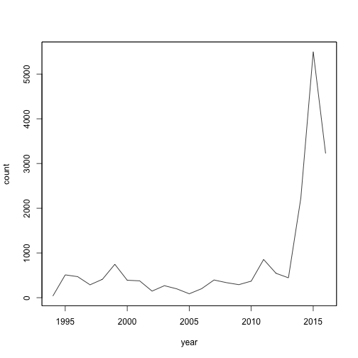

A clear peak in 2015 far beyond anything before. As it seems: In a long-term perspective, 2015 has been the peak of attention for debating refugee migration. For more than two decades.