by Andreas Blätte
The polmineR package uses the rcqp package to access CWB indexed corpora. The core of the rcqp package are R-style C functions wrapping functions of the ‘corpus library’ (CL), a core C library of the CWB. This provides speed. Still, in my feverish dreams, I wondered whether I could access the corpus library directly. As I have installed the CWB, that C library is on my system anyway. Wouldn’t it be nice to be able write my own C routines to call functions of the corpus library?
It does not make sense at all to reimplement the well-developed functionality of the rcqp package. But there are some core bottlenecks in the polmineR package slowing things down. At times, I need to get back and forth between R and the C functions of the corpus library as exposed by rcqp. For these bottlenecks, I have finally managed to implement that old idea of accessing the corpus library directly. In other words, I have written a set of C++ functions for performance critial tasks.
Getting and loading packages
The new C++ code is included in a package I call ‘polmineR.Rcpp’. You may have a look at the package at GitHub and install it from there using devtools. If you want to reproduce things, make sure that you have the latest development version of the polmineR package.
devtools::install_github("PolMine/polmineR.Rcpp")
devtools::install_github("PolMine/polmineR", ref = "dev") # dev to get things from the development branch
We load these two packages, and ggplot2 for visualisation.
library(polmineR)
library(polmineR.Rcpp)
library(ggplot2)
Sufficiently large data
Unsurprisingly, the corpus I use to run some tests is a corpus of protocols of the German Bundestag (“PLPRBT”). A release and an explanation how to use the corpus is planned to supplement the publication of an article I co-authored with Andreas Wüst.
size("PLPRBT")## [1] 100917249It is a 100M corpus. That may be sufficiently large to learn something about performance.
Counting the number of tokens in a corpus
Let us begin with a first standard task, counting the number of tokens in the overall corpus. There are three ways to get there:
- decoding all tokens and counting that;
- obtaining counts from calling the ‘cwb-s-decode’ utility of the CWB, and
- accessing a C function of the corpus library called cqi_id2freq that is not exposed through rcqp but that I can access using Rcpp.
options("polmineR.Rcpp" = TRUE)
Rcpp <- system.time(Corpus$new("PLPRBT")$count(pAttribute = "word"))["elapsed"]
## ... using polmineR.Rcpp for fast countingoptions("polmineR.Rcpp" = FALSE)
options("polmineR.cwb-lexdecode" = TRUE)
lexdecode <- system.time(Corpus$new("PLPRBT")$count(pAttribute = "word"))["elapsed"]## ... using cwb-lexdecode for countingoptions("polmineR.cwb-lexdecode" = FALSE)
base <- system.time(Corpus$new("PLPRBT")$count(pAttribute = "word"))["elapsed"]So let us put things together and look at it.
df <- data.frame(
  method = c("base", "cwb-lexdecode", "Rcpp"),
  time = c(base, lexdecode, Rcpp)
  )
ggplot(df, aes(method, time)) +
  geom_bar(position = "dodge", stat = "identity") +
  ggtitle("Counts for entire corpora") +
  ylab("time (in seconds)")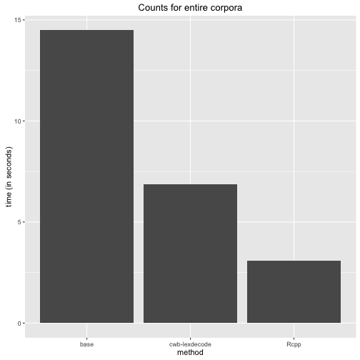
It is fair to say that the cwb-lexdecode utility essentially does the same as the Rcpp function I have written. Time is lost because R will catch the output from the system call and needs to parse it a again into a data.table. Be that as it may. My Rcpp function is the winner.
A helper function
Before I proceed, I introduce a small helper function. To keep the code presented here readable, I decided to work with a wrapper that will execute all functions contained in a list of functions and return the number of seconds it has taken to do that.
getElapsedTime <- function(functions){
  sapply(names(functions), function(x) unname(system.time(functions[[x]]())["elapsed"]))
}
Counting tokens in partitions
The next test concern counts for partitions (i.e. subcorpora) rather than entire corpora. Results will depend on the size of the partition, and I want to compare affairs for corpora of three different kinds: A corpus for one individual speaker (Angela Merkel), for speeches given in one year, and all speeches given in one legislative period. At first, I generate these partitions.
speakerPartition <- partition("PLPRBT", speaker_name = "Angela Merkel")
yearPartition = partition("PLPRBT", speaker_year = "2010")
lpPartition = partition("PLPRBT", speaker_lp = "13")
Let is look at the sizes of these partitions.
size(speakerPartition)## [1] 711414size(yearPartition)## [1] 5910105size(lpPartition)## [1] 17278234So these partitions are as different in size as I wanted them to be. These are the functions that will perform counts for these partitions.
count_functions <- list(
  speaker = function() count(speakerPartition, pAttribute = "word"),
  year = function() count(yearPartition, pAttribute = "word"),
  lp = function() count(lpPartition, pAttribute = "word")
  )
Now, let us run these functions, get the results, doing that with and without Rcpp.
options("polmineR.Rcpp" = FALSE)
noRcpp <- getElapsedTime(count_functions)

options("polmineR.Rcpp" = TRUE)
withRcpp <- getElapsedTime(count_functions)

stats <- rbind(
  data.frame(Rcpp = FALSE, kind = names(noRcpp), values = noRcpp, row.names = NULL),
  data.frame(Rcpp = TRUE, kind = names(withRcpp), values = withRcpp, row.names = NULL)
)
stats$kind <- factor(stats$kind, levels = c("speaker", "year", "lp"))
The following bar chart visualises the results.
ggplot(stats, aes(kind, values, fill = Rcpp)) +
  geom_bar(position = "dodge", stat = "identity") +
  ggtitle("Counting tokens in partitions")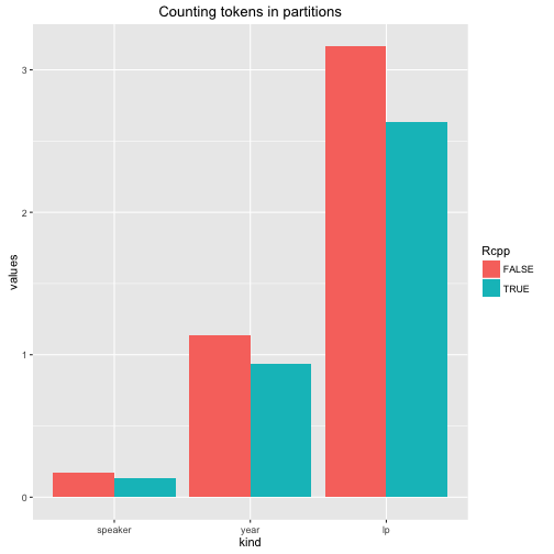
Admittedly, the Rcpp implementation is somewhat faster, but it is not a huge difference.
Creating partitions (without count)
The next scenario is to create a partition, without counts included at first. We do not always need counts. Here are the functions …
partition_without_count <- list(
  speaker = function() partition("PLPRBT", speaker_name = "Angela Merkel"),
  year = function() partition("PLPRBT", speaker_year = "2010"),
  lp = function() partition("PLPRBT", speaker_lp = "13")
  )
Let us execute the functions (with and without Rcpp functions).
options("polmineR.Rcpp" = FALSE)
noRcpp <- getElapsedTime(partition_without_count)

options("polmineR.Rcpp" = TRUE)
withRcpp <- getElapsedTime(partition_without_count)

stats <- rbind(
  data.frame(Rcpp = FALSE, kind = names(noRcpp), values = noRcpp, row.names = NULL),
  data.frame(Rcpp = TRUE, kind = names(withRcpp), values = withRcpp, row.names = NULL)
)
stats$kind <- factor(stats$kind, levels = c("speaker", "year", "lp"))
And here is the bar chart.
ggplot(stats, aes(kind, values, fill = Rcpp)) +
  geom_bar(position = "dodge", stat = "identity") +
  ggtitle("Time consumed for creating partitions")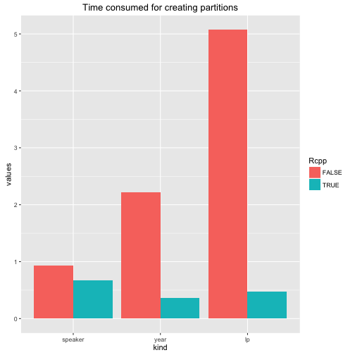
So creating partitions (without counts) is much, much faster.
Faster creation of partitions with counts
The final scenario is the creation of partitions that will include counts. That will be triggered by providing the parameter ‘pAttribute’. We start again with the list of functions…
partition_with_count <- list(
  speaker = function() partition("PLPRBT", speaker_name = "Angela Merkel", pAttribute = "word"),
  year = function() partition("PLPRBT", speaker_year = "2010", pAttribute = "word"),
  lp = function() partition("PLPRBT", speaker_lp = "13", pAttribute = "word")
  )
… run the tests …
options("polmineR.Rcpp" = FALSE)
noRcpp <- getElapsedTime(partition_with_count)

options("polmineR.Rcpp" = TRUE)
withRcpp <- getElapsedTime(partition_with_count)

stats <- rbind(
  data.frame(Rcpp = FALSE, kind = names(noRcpp), time = noRcpp, row.names = NULL),
  data.frame(Rcpp = TRUE, kind = names(withRcpp), time = withRcpp, row.names = NULL)
)
stats$kind <- factor(stats$kind, levels = c("speaker", "year", "lp"))
And we plot the results.
ggplot(stats, aes(kind, time, fill = Rcpp)) +
  geom_bar(position = "dodge", stat = "identity") +
  ggtitle("Time consumed for creating partitions (with counts)")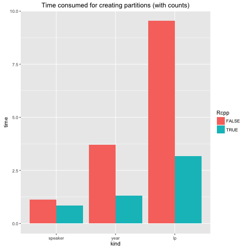
Conclusion
I assume the results are straight forward and do not really need further discussion. There is a lot of talk about the performance gains that can be achieved using Rcpp. Here is the evidence for the polmineR package. Some core functions will run considerably faster.
However, these successes will not induce me to rewrite everything. There are a few other performance boosters in the package. Using the the data.table package has made a huge difference. Still, I am really happy that I managed to write some Rcpp routines that speed up performance critical tasks considerably. It should make using the package more enjoyable!
Subscribe via RSS